Step 3

Step 3 description

The purpose of this configuration is to perform a simulation similar to Step 2 but involving now a mixture of different gaseous species at different temperatures, still without any chemical reaction. In this manner, it is possible to assess the accuracy of the numerical models involved in the description of species and heat diffusion The thermodynamic and transport properties of the 9 species kinetic scheme of Boivin et al. should be used in preparation for the next step, even though the reactions are still neglected here.

It should be noted that in this case, the density is variable in both space and time due to the changing composition, which was not the case in the previous step: this induces additional numerical difficulties that must be taken into account. However, there is no variation of the thermodynamic pressure in time, contrary to the next step.

The simulation domain is a cubic box of size $[0;L]^{3}$ with $L=2\pi L_{0}$ in each direction, where $L_{0}=1\;\mathrm {mm}$. Compared to the previous step, this smaller size is needed to ensure a proper resolution of the reaction fronts for hydrogen oxidation that will appear in the next step and are associated to fixed characteristic dimensions. Again, periodic boundary conditions are used in all three spatial directions.

The initial velocity field prescribed at $t=0$ is identical to the one used in Step 2 with the reference velocity set to $u_{0}=4\;\mathrm {m/s}$.

In preparation for the next step, the central part of the box is initially filled with a $H_{2}/N_{2}$ mixture (fuel region, molar fraction $X_{\mathrm {H_{2}} }^{0}=0.45$, $T=300K$) while the remaining domain is filled with air (oxidizer region, molar fraction $X_{\mathrm {O_{2}} }^{0}=0.21$, $T=300K$). The corresponding mass fractions are $Y_{\mathrm {H_{2}} }^{0}\approx 0.0556$ and $Y_{\mathrm {O_{2}} }^{0}\approx 0.233$.

To avoid any numerical instability, the steps at the interface between both regions are smoothed out using hyperbolic tangent functions as follows:

$R_{d}(x)=|x-0.5\,L|,$ (1)

$\psi (x)=0.5\left[1+\mathrm {tanh} \left({\frac {c\,(R_{d}(x)-R)}{R}}\right)\right],$ (2)

$Y_{\mathrm {H_{2}} }(x)=Y_{\mathrm {H_{2}} }^{0}\left(1-\psi (x)\right),$ (3)

$Y_{\mathrm {O_{2}} }(x)=Y_{\mathrm {O_{2}} }^{0}\left(\psi (x)\right).$ (4)

where $R=\pi /4mm$ and $c=3$ are the half-width of the central slab and stiffness parameter, respectively. As a consequence, there is initially a small region where both fuel and oxidizer coexist. Finally, a nitrogen complement is added everywhere using $Y_{\mathrm {N_{2}} }=1-Y_{\mathrm {H_{2}} }-Y_{\mathrm {O_{2}} }$.

To also test the behaviour of the codes with respect to heat diffusion, a non-homogeneous temperature profile is finally imposed as follows:

• Compute in each cell the equilibrium temperature for the local mixture for constant pressure and enthalpy by using a dedicated solver.

• Enforce the resulting temperature profile, but keep the species profiles to their initial values (Eqs. (3) and (4)).

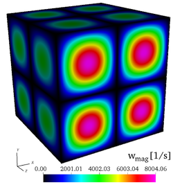
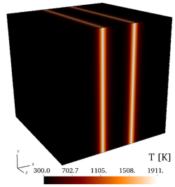
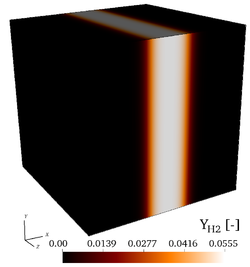
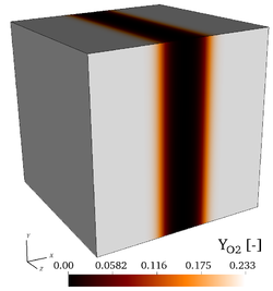
It is found by using Cantera that the peak adiabatic temperature obtained at the fuel/air interface is $T_{ad}=1910.7~K$, leading to the profiles shown in the initial fields of vorticity, temperature, mass fraction of $H_{2}$, mass fraction of $O_{2}$ and the initial profiles of temperature and of mass fractions. Users are encouraged to implement the exact initial profiles from the benchmark website to facilitate later comparisons.

The resulting, initial configuration thus involves multiple species at different temperatures with steep profiles, just like in a real flame. However, for the present simulation, the reaction source terms are all still set to zero, as already mentioned: only convection and diffusion processes are considered. In order to enable benchmark computations also with DNS codes that do not provide advanced diffusion models, only constant values of the Lewis numbers are considered; for the same reason, thermodiffusion (Soret effect) is neglected on purpose (though it would be obviously relevant for such cases involving hydrogen as a fuel). The authors are fully aware that this is a crude approximation of reality. But it must be kept in mind that the focus is set here on the detailed comparison between different codes and algorithms, and not on the resulting flow or flame structure. Hence, in this and in the next section, the values of the Lewis number for each species given in the table below shall be used to enable direct comparisons. These values have been estimated from a separate DNS for a similar configuration using the mixture-averaged diffusion model. The precise description of the associated thermodynamic state is available on the website.

Approximate Lewis number for the species appearing in the kinetic scheme of, to be enforced for Step 3 and Step 4 of the benchmark

Species	$H_{2}$	$H$	$O_{2}$	$OH$	$O$	$H_{2}O$	$HO_{2}$	$H_{2}O_{2}$	$N_{2}$
Lewis number	0.3290	0.2228	1.2703	0.8279	0.8128	1.0741	1.2582	1.2665	1.8268

On the other hand, considering that implementing advanced models for fluid viscosity and thermal conductivity is not difficult and does not increase the computational time significantly, local values of these quantities depending on composition and temperature should be taken into account; More specifically, and to ease further comparisons, the same models for viscosity and conductivity have been retained in the three participating codes, i.e. the mixture averaged formalism that is used in both the Cantera and Chemkin packages. More details on these models are available on the benchmark repository, such as reference data for viscosity and conductivity along various cuts at initialization.

The viscosity is variable in the computational domain as well as with time and the Reynolds number of this configuration can only be estimated using the minimal value of viscosity (which is obtained in the air at 300 K, $\nu _{\mathrm {min} }\approx 1.56\,10^{-5}\mathrm {m^{2}/s}$), leading to $Re={u_{0}L_{0}}/{\nu _{min}}=267$ which guarantees a laminar flow.

Concerning resolution, it is also suggested to keep a conservative resolution in time for this benchmark, corresponding to $CFL\leq 0.25$ and $Fo\leq 0.15$. In space, each direction should be resolved by approximately 256 grid points, leading to a spatial resolution $\Delta x\approx 25\mu m$.

The reference time scale is here $\tau _{\mathrm {ref} }=L_{0}/u_{0}=0.25\;\mathrm {ms}$. The simulation should be performed for a physical time of at least $t=0.5\;\mathrm {ms} =2\tau _{\mathrm {ref} }$ as most of the results presented in this article are taken from this instant. Data up to $t=2.5\;\mathrm {ms} =10\tau _{\mathrm {ref} }$ are available on the benchmark repository.

Initial fields of vorticity magnitude, temperature, mass fractions of $\mathrm {H_{2}}$, and mass fraction of $\mathrm {O_{2}}$ (from left to right), for the 3-D, non-reacting case (Step 3).

File:Profiles 3d zoom.pdf

Initial profiles of temperature and of mass fractions at $y=0.5L$ and $z=0.5L$ for the 3-D, non-reacting case (Step 3).

Kinetics

The Boivin scheme [1] has been used for this Benchmark.

[2] [3]

Reference: P. Boivin, C. Jiménez, A.L. Sánchez, F.A. Williams, An explicit reduced mechanism for H2–air combustion, Proceedings of the Combustion Institute, Volume 33, Issue 1, 2011, Pages 517-523, ISSN 1540-7489,

Transport and thermodynamic properties used for this Step

\cf{I think we all used the same transport (viscosity) and thermodynamic properties, but we should check again and compare that the implementations used in cantera/Chemkin provide the same values.}

\gl{Good idea: we could use 3 or 4 relevant reference compositions to quantify the discrepancies between Cantera and Chemkin (on rho, Cp, conductivity, viscosity for example) and also put these on the website.}

Put the transport data here

Aside suggestions

TBD