Analysis of Step 3

The main difference between this step and the previous one, is that now species and heat diffusion are additionally taken into account in an inhomogeneous environment. Neither analytical nor reference solution are available for this configuration, so that only comparisons between the three codes involved in the benchmark are possible. Compared to Step 2, the presence of high-temperature regions additionally modifies the evolution of the TGV with time, turbulence being locally damped due to dilatation and higher viscosities. As a consequence, the needed resolution for this case is less than in Step 2: YALES2 and DINO used only 256 grid points in each direction while Nek5000 used 36 elements (again with 7 Gauss-Lobatto-Legendre points in each element), i.e. 252 points in each direction.

The results that will be compared involve:

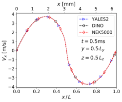
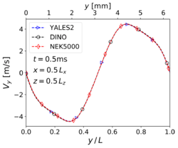
1. Velocity profiles at $t=2\tau _{ref}=0.5ms$ along the centerlines of the domain;

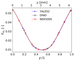
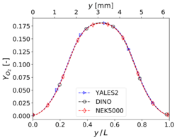
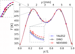
2. Profiles of $H_{2}$ and $O_{2}$ mass fractions and profile of temperature at $t=2\tau _{ref}=0.5ms$ along the y-centerline of the domain;

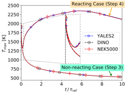
3. Evolution of maximal temperature in the domain vs. time.

Looking at the results of velocity at time $t=2\tau _{ref}=0.5ms$ along the centerlines of the computational domain, it is observed that the three codes deliver the same velocity profiles; the agreement is visually perfect. The results for the two main species mass fractions ($Y_{H2}$ and $Y_{O2}$) are also in excellent agreement among the three participating codes.

Profile of mass fractions of $H_{2}$ (left) and $O_{2}$ (right) at $t=2\tau _{ref}ms$, $x=0.5L$, and $z=0.5L$ for 3-D non-reacting multi-species flow (Step 3).

Regarding temperature, the figure on the left shows along the centerline two peaks and one valley, as expected. Very small deviations are revealed in the inlaid enlargements shown in this figure. Finally, the evolution with time of maximum temperature inside the computational domain is presented in the figure on the right. Here again, no differences are observed at all concerning this parameter. As a conclusion concerning this step, the three codes are able to reproduce numerically the behavior of a complex multi-species, non-isothermal flow with excellent agreement, and are thus strong candidates for high-fidelity simulations of turbulent flames, as considered in the next and final step.