Difference between revisions of "Analysis of Step 4"
| (15 intermediate revisions by the same user not shown) | |||
| Line 1: | Line 1: | ||
| − | '''Step 4''' is definitely the most complex but also the most interesting case to compare '''high-fidelity codes''' for '''turbulent | + | '''Step 4''' is definitely the most complex but also the most interesting case to compare '''high-fidelity codes''' for '''turbulent reacting flows''', since it contains all the features relevant for '''turbulent combustion'''. Therefore, a more detailed analysis is useful. The comparisons will involve: |
| − | reacting flows''', since it contains all the features relevant for '''turbulent combustion'''. Therefore, a more detailed analysis | + | |
| − | is useful. The comparisons will involve: | + | |
| − | 1. The evolution of maximum temperature versus time | + | 1. The '''evolution of maximum temperature''' versus '''time'''; |
| − | 2. Velocity fields at <math>t = 2 \tau_{ref} = 0.5 ms</math> along the centerlines of the domain | + | 2. '''Velocity fields''' at <math>t = 2 \tau_{ref} = 0.5 ms</math> along the centerlines of the domain; |
| − | 3. Profiles of temperature, heat release and mass fractions of | + | 3. '''Profiles of temperature''', '''heat release''' and '''mass fractions''' of <math>H_2</math>, <math>O_2</math> and <math>OH</math> at <math>t = 2 \tau_{ref} = 0.5 ms</math> along the centerline of the domain. |
| − | centerline of the domain | + | |
The simulations of '''YALES2''', '''DINO''' and '''Nek5000''' are presented in the following subsections for two different | The simulations of '''YALES2''', '''DINO''' and '''Nek5000''' are presented in the following subsections for two different | ||
| − | resolutions in space ( | + | resolutions in space (<math>256^3</math> and <math>512^3</math>), in order to check the impact of the '''spatial resolution''' on the results. Additional data for other grids are also available (<math>384^3</math> |
| − | ), in order to check the impact of the '''spatial resolution''' on the results. Additional | + | for both '''YALES2''' and '''DINO''', and <math>768^3</math> only for '''DINO'''). They are not discussed at length in the text and in separate figures in the interest of space, but the corresponding values are included in the Tables 4 and 5 summarizing all results of '''Step 4'''. Additionally, all results at all grid resolutions are available online in the benchmark repository <ref name="TGV-coria-cfd">[https://benchmark.coria-cfd.fr benchmark.coria-cfd.fr]</ref>. |
| − | data for other grids are also available ( | + | |
| − | for both '''YALES2''' and '''DINO''', and | + | |
| − | discussed at length in the text and in separate figures in the interest of space, but the corresponding values are | + | |
| − | included in the Tables 4 and 5 summarizing all results of '''Step 4'''. Additionally, all results at all grid resolutions are | + | |
| − | available online in the benchmark repository [ | + | |
Starting with the evolution of maximum temperature versus time, a perfect visual agreement between all three | Starting with the evolution of maximum temperature versus time, a perfect visual agreement between all three | ||
| − | codes is observed at all resolutions | + | codes is observed at all resolutions. This quantity does not appear to be difficult to predict correctly, as already observed previously for the non-reacting flow in '''Step 3''', provided that the pressure variation due to the heat release is correctly taken into account. |
| − | + | ||
| − | to be difficult to predict correctly, as already observed previously for the non-reacting flow in '''Step 3''', provided that the pressure variation due to the heat release is correctly taken into account. | + | |
== Comparing results at spatial resolution of <math>256^3</math> == | == Comparing results at spatial resolution of <math>256^3</math> == | ||
| − | The results shown in this section have been obtained for the same grid size than in '''Step 3''', i.e. | + | The results shown in this section have been obtained for the same grid size than in '''Step 3''', i.e. <math>256^3</math> |
for '''YALES2''' | for '''YALES2''' | ||
and '''DINO''' and 2523 | and '''DINO''' and 2523 | ||
| − | for '''Nek5000'''. The corresponding results for '''velocity''' | + | for '''Nek5000'''. The corresponding results for '''velocity''' and '''temperature''' at time <math>t = 2 \tau_{ref} = 0.5 ms</math> along the centerlines of the domain show visually a perfect agreement. Nevertheless, the three codes show slight differences concerning heat release and some '''mass fractions profiles''' (in particular <math>O_2</math> and <math>OH</math>) around the center of the domain. These differences – though small |
| − | at time <math>t = 2 \tau_{ref} = 0.5 ms</math> along the centerlines of the domain show visually a perfect agreement. Nevertheless, the | + | |
| − | three codes show slight differences concerning heat release and some '''mass fractions profiles''' (in particular <math>O_2</math> and <math>OH</math>) | + | |
| − | around the center of the domain | + | |
– are larger than those experienced in the non-reacting case. Note that there is originally no oxygen in this region, | – are larger than those experienced in the non-reacting case. Note that there is originally no oxygen in this region, | ||
explaining why the mass fraction of <math>O_2</math> is still smaller than the mass fraction of <math>OH</math> there. One reason behind these | explaining why the mass fraction of <math>O_2</math> is still smaller than the mass fraction of <math>OH</math> there. One reason behind these | ||
| Line 39: | Line 26: | ||
case, the typical cell size is approximately 25 µm. To check this last point, the simulations have been repeated with | case, the typical cell size is approximately 25 µm. To check this last point, the simulations have been repeated with | ||
a finer spatial resolution, as discussed in the next subsection. | a finer spatial resolution, as discussed in the next subsection. | ||
| + | |||
| + | [[File:vx_x_lm_256.png|250px]] | ||
| + | [[File:vy_y_lm_256.png|250px]] | ||
| + | |||
| + | '''Velocity''' at time <math>t = 2τref = 0.5 ms</math> for '''3-D reacting case''' ('''Step 4''') with <math>N = 256^3</math> grid points. | ||
| + | |||
| + | [[File:T_y_lm_256.png|250px]] | ||
| + | [[File:hr_y_lm_256_withzoom.png|250px]] | ||
| + | |||
| + | '''Temperature''' (left) and '''heat release profiles''' (right) at <math>x = 0.5 L</math>, <math>z = 0.5 L</math>, and time <math>t = 2 \tau_{ref} = 0.5 ms</math> for '''3-D reacting case''' | ||
| + | ('''Step 4''') with <math>N = 256^3</math> grid points. | ||
| + | |||
| + | [[File:yh2_y_lm_256.png|250px]] | ||
| + | [[File:yo2_y_lm_256_withzoom.png|250px]] | ||
| + | [[File:yoh_y_lm_256_withzoom.png|250px]] | ||
| + | |||
| + | '''Mass fraction profiles''' of <math>H_2</math>, <math>O_2</math>, and <math>OH</math> at </math>x = 0.5 L</math>, <math>z = 0.5 L</math>, and time <math>t = 2\tau_{ref} = 0.5 ms</math> for 3-D reacting case (Step 4) | ||
| + | with <math>N = 256^3</math> grid points. | ||
== Comparing results at spatial resolution of <math>512^3</math> == | == Comparing results at spatial resolution of <math>512^3</math> == | ||
| − | The present results have been obtained on a grid size of | + | The present results have been obtained on a grid size of <math>512^3</math> for '''YALES2''' and '''DINO''', while '''Nek5000''' relies on |
| − | for '''YALES2''' and '''DINO''', while '''Nek5000''' relies on | + | |
similar '''discretization''' size of 5143 | similar '''discretization''' size of 5143 | ||
(57 '''spectral elements''' of order 9 in each direction). To reduce computational costs, | (57 '''spectral elements''' of order 9 in each direction). To reduce computational costs, | ||
the simulation is conducted only for the first <math>t = 2 \tau_{ref} = 0.5 ms</math> of physical time. | the simulation is conducted only for the first <math>t = 2 \tau_{ref} = 0.5 ms</math> of physical time. | ||
| − | Only the quantities showing visible discrepancies at a resolution of | + | Only the quantities showing visible discrepancies at a resolution of <math>256^3</math> |
| − | (heat release, <math>Y_{O_2}</math> | + | (heat release, <math>Y_{O_2}</math>, <math>Y_{OH}</math>) are discussed here in the interest of brevity, since all other quantities already revealed a perfect agreement for the previous resolution. |
| − | , <math>Y_{OH}</math>) are discussed here | + | It can be observed in the figures below that doubling the spatial resolution in each direction did not improve the |
| − | in the interest of brevity, since all other quantities already revealed a perfect agreement for the previous resolution. | + | |
| − | It can be observed in | + | |
comparisons in a clear way; marginal differences still exist between the codes, and a convergence towards a unique | comparisons in a clear way; marginal differences still exist between the codes, and a convergence towards a unique | ||
solution is not really visible. To discuss this issue in more detail, a refined analysis is necessary, as discussed in the | solution is not really visible. To discuss this issue in more detail, a refined analysis is necessary, as discussed in the | ||
next subsection. | next subsection. | ||
| + | |||
| + | [[File:T_y_lm_512.png|250px]] | ||
| + | [[File:hr_y_lm_512_withzoom.png|250px]] | ||
| + | |||
| + | '''Temperature''' (left) and '''heat release profiles''' (right) at <math>x = 0.5 L</math>, <math>z = 0.5 L</math>, and time <math>t = 2 \tau_{ref} = 0.5 ms</math> for '''3-D reacting case''' ('''Step 4''') with <math>N = 512^3</math> grid points. | ||
| + | |||
| + | [[File:yo2_y_lm_512_withzoom.png|250px]] | ||
| + | [[File:yoh_y_lm_512_withzoom.png|250px]] | ||
| + | |||
| + | '''Mass fraction profiles''' of <math>O_2</math> (left), and <math>OH</math> (right) at <math>x = 0.5 L</math>, <math>z = 0.5 L</math>, and time <math>t = 2 \tau_{ref} = 0.5 ms</math> for '''3-D reacting case''' | ||
| + | ('''Step 4''') with <math>N = 512^3</math> grid points. | ||
== Quantitative comparisons at the center point at t = 0.5 ms == | == Quantitative comparisons at the center point at t = 0.5 ms == | ||
| Line 64: | Line 77: | ||
corresponding value) is also listed in the table; it depends on the retained criteria and on the explicit or implicit | corresponding value) is also listed in the table; it depends on the retained criteria and on the explicit or implicit | ||
integration of the corresponding terms in the equations. | integration of the corresponding terms in the equations. | ||
| + | |||
| + | {| class="wikitable alternance center" | ||
| + | |+ Values of different variables at the center of the domain at time <math>t = 2 \tau_{ref} = 0.5 ms</math> | ||
| + | |- | ||
| + | ! scope="row" | Code | ||
| + | | YALES2 | ||
| + | | YALES2 | ||
| + | | YALES2 | ||
| + | | DINO | ||
| + | | DINO | ||
| + | | DINO | ||
| + | | DINO | ||
| + | | Nek5000 | ||
| + | | Nek5000 | ||
| + | |- | ||
| + | ! scope="row" | Spatial resolution | ||
| + | | <math>256^3</math> | ||
| + | | <math>384^3</math> | ||
| + | | <math>512^3</math> | ||
| + | | <math>256^3</math> | ||
| + | | <math>384^3</math> | ||
| + | | <math>512^3</math> | ||
| + | | <math>768^3</math> | ||
| + | | <math>252^3</math> | ||
| + | | <math>504^3</math> | ||
| + | |- | ||
| + | ! scope="row" | Timestep control | ||
| + | | CFL=0.10 | ||
| + | | CFL=0.15 | ||
| + | | CFL=0.25 | ||
| + | | Fo=0.15 | ||
| + | | Fo=0.15 | ||
| + | | Fo=0.15 | ||
| + | | Fo=0.2 | ||
| + | | CFL=0.25 | ||
| + | | CFL=0.25 | ||
| + | |- | ||
| + | ! scope="row" | <math>T[K]</math> | ||
| + | | 1752 | ||
| + | | 1751 | ||
| + | | 1750 | ||
| + | | 1754 | ||
| + | | 1755 | ||
| + | | 1755 | ||
| + | | 1758 | ||
| + | | 1758 | ||
| + | | 1758 | ||
| + | |- | ||
| + | ! scope="row" | <math>Y_{O_2}[-]</math> | ||
| + | | 1.553E-3 | ||
| + | | 1.523E-3 | ||
| + | | 1.523E-3 | ||
| + | | 1.508E-3 | ||
| + | | 1.500E-3 | ||
| + | | 1.508E-3 | ||
| + | | 1.521E-3 | ||
| + | | 1.499E-3 | ||
| + | | 1.506E-3 | ||
| + | |- | ||
| + | ! scope="row" | <math>Y_{H_2}[-]</math> | ||
| + | | 2.692E-3 | ||
| + | | 2.714E-3 | ||
| + | | 2.720E-3 | ||
| + | | 2.764E-3 | ||
| + | | 2.737E-3 | ||
| + | | 2.720E-3 | ||
| + | | 2.700E-3 | ||
| + | | 2.681E-3 | ||
| + | | 2.688E-3 | ||
| + | |- | ||
| + | ! scope="row" | <math>Y_{OH}[-]</math> | ||
| + | | 1.852E-3 | ||
| + | | 1.838E-3 | ||
| + | | 1.831E-3 | ||
| + | | 1.844E-3 | ||
| + | | 1.851E-3 | ||
| + | | 1.858E-3 | ||
| + | | 1.873E-3 | ||
| + | | 1.862E-3 | ||
| + | | 1.861E-3 | ||
| + | |- | ||
| + | ! scope="row" | <math>HR[MW/m^3]</math> | ||
| + | | 670.8 | ||
| + | | 669.7 | ||
| + | | 670.1 | ||
| + | | 684.1 | ||
| + | | 675.8 | ||
| + | | 673.5 | ||
| + | | 671.8 | ||
| + | | 674.2 | ||
| + | | 660.8 | ||
| + | |} | ||
Looking separately at the values obtained by each code, it is not always easy to recognize the convergence toward | Looking separately at the values obtained by each code, it is not always easy to recognize the convergence toward | ||
| Line 71: | Line 176: | ||
This is why, choosing arbitrarily the results of the implicit time integration at the highest spatial resolution with | This is why, choosing arbitrarily the results of the implicit time integration at the highest spatial resolution with | ||
'''DINO''' (7683) as a reference, all corresponding relative errors have been computed. | '''DINO''' (7683) as a reference, all corresponding relative errors have been computed. | ||
| + | |||
| + | {| class="wikitable alternance center" | ||
| + | |+ Values of different variables at the center of the domain at time <math>t = 2 \tau_{ref} = 0.5 ms</math> | ||
| + | |- | ||
| + | ! scope="row" | Code | ||
| + | | YALES2 | ||
| + | | YALES2 | ||
| + | | YALES2 | ||
| + | | DINO | ||
| + | | DINO | ||
| + | | DINO | ||
| + | | DINO | ||
| + | | Nek5000 | ||
| + | | Nek5000 | ||
| + | |- | ||
| + | ! scope="row" | Spatial resolution | ||
| + | | <math>256^3</math> | ||
| + | | <math>384^3</math> | ||
| + | | <math>512^3</math> | ||
| + | | <math>256^3</math> | ||
| + | | <math>384^3</math> | ||
| + | | <math>512^3</math> | ||
| + | | <math>768^3</math> | ||
| + | | <math>253^3</math> | ||
| + | | <math>514^3</math> | ||
| + | |- | ||
| + | ! scope="row" | Controlling CFL/Fo | ||
| + | | CFL=0.10 | ||
| + | | CFL=0.15 | ||
| + | | CFL=0.25 | ||
| + | | Fo=0.15 | ||
| + | | Fo=0.15 | ||
| + | | Fo=0.15 | ||
| + | | Fo=0.2 | ||
| + | | CFL=0.25 | ||
| + | | CFL=0.25 | ||
| + | |- | ||
| + | ! scope="row" | <math>\Delta T[%]</math> | ||
| + | | −0.341 | ||
| + | | −0.398 | ||
| + | | −0.455 | ||
| + | | −0.228 | ||
| + | | −0.171 | ||
| + | | −0.171 | ||
| + | | 0 [Ref] | ||
| + | | 0 | ||
| + | | 0 | ||
| + | |- | ||
| + | ! scope="row" | <math>\Delta Y_{O_2}[%]</math> | ||
| + | | 2.104 | ||
| + | | 0.131 | ||
| + | | 0.131 | ||
| + | | −0.855 | ||
| + | | −1.381 | ||
| + | | −0.855 | ||
| + | | 0 [Ref] | ||
| + | | −1.446 | ||
| + | | −0.986 | ||
| + | |- | ||
| + | ! scope="row" | <math>\Delta Y_{H_2}[%]</math> | ||
| + | | −0.296 | ||
| + | | 0.518 | ||
| + | | 0.741 | ||
| + | | 2.370 | ||
| + | | 1.370 | ||
| + | | 0.741 | ||
| + | | 0 [Ref] | ||
| + | | −0.704 | ||
| + | | −0.444 | ||
| + | |- | ||
| + | ! scope="row" | <math>\Delta Y_{OH}[%]</math> | ||
| + | | −1.121 | ||
| + | | −1.869 | ||
| + | | −2.242 | ||
| + | | −1.548 | ||
| + | | −1.175 | ||
| + | | −0.801 | ||
| + | | 0 [Ref] | ||
| + | | −0.587 | ||
| + | | −0.641 | ||
| + | |- | ||
| + | ! scope="row" | <math>\Delta HR[%]</math> | ||
| + | | −0.149 | ||
| + | | −0.313 | ||
| + | | −0.253 | ||
| + | | 1.831 | ||
| + | | 0.595 | ||
| + | | 0.253 | ||
| + | | 0 [Ref] | ||
| + | | 0.363 | ||
| + | | −1.637 | ||
| + | |} | ||
Analyzing in detail all the values, the following intermediate conclusions can be drawn: | Analyzing in detail all the values, the following intermediate conclusions can be drawn: | ||
| Line 84: | Line 281: | ||
• Increasing further the '''spatial resolution''' (which is also connected to a '''reduction of the timestep''') does not seem | • Increasing further the '''spatial resolution''' (which is also connected to a '''reduction of the timestep''') does not seem | ||
to increase much the observed agreement between the codes. For all considered grids in the analysis finer | to increase much the observed agreement between the codes. For all considered grids in the analysis finer | ||
| − | than | + | than <math>256^3</math>, overall differences of the order of 1% are observed. Often, using a finer resolution leads to a better |
agreement for most of the indicators, but to a worse comparison for some other ones. | agreement for most of the indicators, but to a worse comparison for some other ones. | ||
• Though this has been attempted, it was impossible to obtain meaningful predictions using the '''Richardson | • Though this has been attempted, it was impossible to obtain meaningful predictions using the '''Richardson | ||
| − | extrapolation''' | + | extrapolation''' <ref name="Ferziger2012"/><ref name="Celik2008"/>, since the results of all codes are '''non-monotonic''' when increasing resolution in space. |
• Somewhat unexpectedly, the '''observed uncertainty is in the same range for temperature, mass fractions of main | • Somewhat unexpectedly, the '''observed uncertainty is in the same range for temperature, mass fractions of main | ||
| Line 94: | Line 291: | ||
Finally, the central finding is that all codes employed in the benchmark deliver suitable results for this configuration, | Finally, the central finding is that all codes employed in the benchmark deliver suitable results for this configuration, | ||
| − | and this already at a typical grid resolution of | + | and this already at a typical grid resolution of <math>256^3</math> |
for this particular case. An irreducible uncertainty of the order | for this particular case. An irreducible uncertainty of the order | ||
of 1% is observed for all quantities relevant for turbulent combustion. This uncertainty, noticeably larger than for | of 1% is observed for all quantities relevant for turbulent combustion. This uncertainty, noticeably larger than for | ||
| Line 100: | Line 297: | ||
libraries/library versions employed for computing thermodynamic, diffusion, and reaction parameters. | libraries/library versions employed for computing thermodynamic, diffusion, and reaction parameters. | ||
After this detailed analysis of uncertainty, '''it is necessary to quantify the corresponding numerical costs needed to get this level of accuracy.''' | After this detailed analysis of uncertainty, '''it is necessary to quantify the corresponding numerical costs needed to get this level of accuracy.''' | ||
| + | |||
| + | = References = | ||
| + | |||
| + | <references> | ||
| + | <ref name="Ferziger2012"> | ||
| + | <bibtex> | ||
| + | @article{Ferziger2012, | ||
| + | author= {J.H. Ferziger and M. Peric}, | ||
| + | title= {Computational Methods for Fluid Dynamics}, | ||
| + | journal={Springer}, | ||
| + | year= {2012}, | ||
| + | } | ||
| + | </bibtex> | ||
| + | </ref> | ||
| + | <ref name="Celik2008"> | ||
| + | <bibtex> | ||
| + | @article{Celik2008, | ||
| + | author= {I.B. Celik, U. Ghia, P.J. Roache, C.J. Freitas, H. Coleman, and P.E. Raad}, | ||
| + | title= {Procedure for estimation and | ||
| + | reporting of uncertainty due to discretization in CFD applications}, | ||
| + | journal={J. Fluids Eng.}, | ||
| + | year= {2008}, | ||
| + | volume={130}, | ||
| + | } | ||
| + | </bibtex> | ||
| + | </ref> | ||
| + | </references> | ||
Latest revision as of 15:33, 26 August 2020
Step 4 is definitely the most complex but also the most interesting case to compare high-fidelity codes for turbulent reacting flows, since it contains all the features relevant for turbulent combustion. Therefore, a more detailed analysis is useful. The comparisons will involve:
1. The evolution of maximum temperature versus time;
2. Velocity fields at along the centerlines of the domain;
3. Profiles of temperature, heat release and mass fractions of , and at along the centerline of the domain.
The simulations of YALES2, DINO and Nek5000 are presented in the following subsections for two different resolutions in space ( and ), in order to check the impact of the spatial resolution on the results. Additional data for other grids are also available ( for both YALES2 and DINO, and only for DINO). They are not discussed at length in the text and in separate figures in the interest of space, but the corresponding values are included in the Tables 4 and 5 summarizing all results of Step 4. Additionally, all results at all grid resolutions are available online in the benchmark repository [1]. Starting with the evolution of maximum temperature versus time, a perfect visual agreement between all three codes is observed at all resolutions. This quantity does not appear to be difficult to predict correctly, as already observed previously for the non-reacting flow in Step 3, provided that the pressure variation due to the heat release is correctly taken into account.
Contents
Comparing results at spatial resolution of
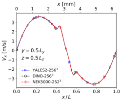
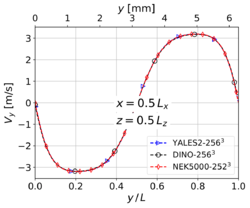
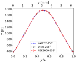
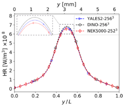
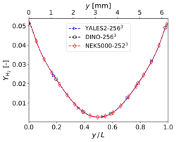
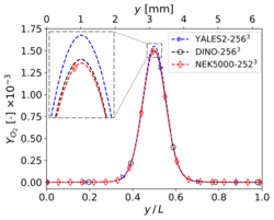
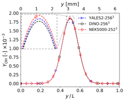
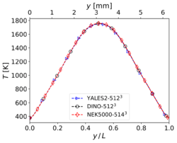
The results shown in this section have been obtained for the same grid size than in Step 3, i.e. for YALES2 and DINO and 2523 for Nek5000. The corresponding results for velocity and temperature at time along the centerlines of the domain show visually a perfect agreement. Nevertheless, the three codes show slight differences concerning heat release and some mass fractions profiles (in particular and ) around the center of the domain. These differences – though small – are larger than those experienced in the non-reacting case. Note that there is originally no oxygen in this region, explaining why the mass fraction of is still smaller than the mass fraction of there. One reason behind these discrepancies might be the well-known stiffness of the chemical source terms, inducing different non-linear effects as a function of the underlying algorithms employed for integration in time. Another possible source of error is the employed spatial discretization, which might still be insufficient to perfectly capture the reaction front; in the present case, the typical cell size is approximately 25 µm. To check this last point, the simulations have been repeated with a finer spatial resolution, as discussed in the next subsection.
Velocity at time for 3-D reacting case (Step 4) with grid points.
Temperature (left) and heat release profiles (right) at , , and time for 3-D reacting case (Step 4) with grid points.
Mass fraction profiles of , , and at </math>x = 0.5 L</math>, , and time for 3-D reacting case (Step 4) with grid points.
Comparing results at spatial resolution of
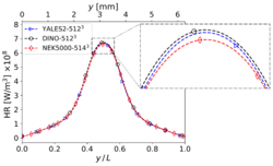
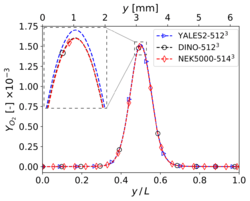
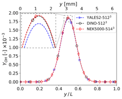
The present results have been obtained on a grid size of for YALES2 and DINO, while Nek5000 relies on similar discretization size of 5143 (57 spectral elements of order 9 in each direction). To reduce computational costs, the simulation is conducted only for the first of physical time. Only the quantities showing visible discrepancies at a resolution of (heat release, , ) are discussed here in the interest of brevity, since all other quantities already revealed a perfect agreement for the previous resolution. It can be observed in the figures below that doubling the spatial resolution in each direction did not improve the comparisons in a clear way; marginal differences still exist between the codes, and a convergence towards a unique solution is not really visible. To discuss this issue in more detail, a refined analysis is necessary, as discussed in the next subsection.
Temperature (left) and heat release profiles (right) at , , and time for 3-D reacting case (Step 4) with grid points.
Mass fraction profiles of (left), and (right) at , , and time for 3-D reacting case (Step 4) with grid points.
Quantitative comparisons at the center point at t = 0.5 ms
In Table 4 the values of different variables at the center of the numerical domain at time are presented and analyzed. These values have been obtained for the three different codes involved in the benchmark (from left to right, YALES2, DINO, Nek5000), for an increasing spatial resolution from left to right, but also with different timesteps. The controlling time-limiter (as a condition on maximum CFL or Fourier number with corresponding value) is also listed in the table; it depends on the retained criteria and on the explicit or implicit integration of the corresponding terms in the equations.
| Code | YALES2 | YALES2 | YALES2 | DINO | DINO | DINO | DINO | Nek5000 | Nek5000 |
|---|---|---|---|---|---|---|---|---|---|
| Spatial resolution | |||||||||
| Timestep control | CFL=0.10 | CFL=0.15 | CFL=0.25 | Fo=0.15 | Fo=0.15 | Fo=0.15 | Fo=0.2 | CFL=0.25 | CFL=0.25 |
| 1752 | 1751 | 1750 | 1754 | 1755 | 1755 | 1758 | 1758 | 1758 | |
| 1.553E-3 | 1.523E-3 | 1.523E-3 | 1.508E-3 | 1.500E-3 | 1.508E-3 | 1.521E-3 | 1.499E-3 | 1.506E-3 | |
| 2.692E-3 | 2.714E-3 | 2.720E-3 | 2.764E-3 | 2.737E-3 | 2.720E-3 | 2.700E-3 | 2.681E-3 | 2.688E-3 | |
| 1.852E-3 | 1.838E-3 | 1.831E-3 | 1.844E-3 | 1.851E-3 | 1.858E-3 | 1.873E-3 | 1.862E-3 | 1.861E-3 | |
| 670.8 | 669.7 | 670.1 | 684.1 | 675.8 | 673.5 | 671.8 | 674.2 | 660.8 |
Looking separately at the values obtained by each code, it is not always easy to recognize the convergence toward a single value that would be expected for a grid-independence analysis. By a comparison between the last column for each code, a good agreement is overall observed, in spite of differences regarding algorithms, resolution in space and in time. Nevertheless, the agreement is never perfect, and trends can better be seen by computing differences. This is why, choosing arbitrarily the results of the implicit time integration at the highest spatial resolution with DINO (7683) as a reference, all corresponding relative errors have been computed.
| Code | YALES2 | YALES2 | YALES2 | DINO | DINO | DINO | DINO | Nek5000 | Nek5000 |
|---|---|---|---|---|---|---|---|---|---|
| Spatial resolution | |||||||||
| Controlling CFL/Fo | CFL=0.10 | CFL=0.15 | CFL=0.25 | Fo=0.15 | Fo=0.15 | Fo=0.15 | Fo=0.2 | CFL=0.25 | CFL=0.25 |
| −0.341 | −0.398 | −0.455 | −0.228 | −0.171 | −0.171 | 0 [Ref] | 0 | 0 | |
| 2.104 | 0.131 | 0.131 | −0.855 | −1.381 | −0.855 | 0 [Ref] | −1.446 | −0.986 | |
| −0.296 | 0.518 | 0.741 | 2.370 | 1.370 | 0.741 | 0 [Ref] | −0.704 | −0.444 | |
| −1.121 | −1.869 | −2.242 | −1.548 | −1.175 | −0.801 | 0 [Ref] | −0.587 | −0.641 | |
| −0.149 | −0.313 | −0.253 | 1.831 | 0.595 | 0.253 | 0 [Ref] | 0.363 | −1.637 |
Analyzing in detail all the values, the following intermediate conclusions can be drawn:
• The overall agreement between the three completely independent high-resolution codes employed in the benchmark is very good, with typical relative differences of the order of 1% for the essential quantities used to analyze turbulent combustion (temperature, mass fractions, heat release). 23
• Compared to the differences observed in the previous verification step (errors below 0.03%), the variations are obviously much larger, typically by two orders of magnitude. This is a result of the far more challenging configuration, with additional physicochemical complexity, stiffer profiles, highly non-linear processes in space and time.
• Increasing further the spatial resolution (which is also connected to a reduction of the timestep) does not seem to increase much the observed agreement between the codes. For all considered grids in the analysis finer than , overall differences of the order of 1% are observed. Often, using a finer resolution leads to a better agreement for most of the indicators, but to a worse comparison for some other ones.
• Though this has been attempted, it was impossible to obtain meaningful predictions using the Richardson extrapolation [2][3], since the results of all codes are non-monotonic when increasing resolution in space.
• Somewhat unexpectedly, the observed uncertainty is in the same range for temperature, mass fractions of main species or of radicals, and heat release. Quantities that are typically considered more sensitive (radicals, heat release) do not lead to larger discrepancies in the analysis.
Finally, the central finding is that all codes employed in the benchmark deliver suitable results for this configuration, and this already at a typical grid resolution of for this particular case. An irreducible uncertainty of the order of 1% is observed for all quantities relevant for turbulent combustion. This uncertainty, noticeably larger than for cold flows, is apparently the result of stiff non-linear processes, of different splitting schemes, and of the different libraries/library versions employed for computing thermodynamic, diffusion, and reaction parameters. After this detailed analysis of uncertainty, it is necessary to quantify the corresponding numerical costs needed to get this level of accuracy.
References
- ↑ benchmark.coria-cfd.fr
- ↑
J.H. Ferziger, M. Peric, Computational Methods for Fluid Dynamics, Springer , 2012, BibtexAuthor : J.H. Ferziger, M. Peric
Title : Computational Methods for Fluid Dynamics
In : Springer -
Address :
Date : 2012 - ↑
I.B. Celik, U. Ghia, P.J. Roache, C.J. Freitas, H. Coleman,, P.E. Raad, Procedure for estimation and
reporting of uncertainty due to discretization in CFD applications, J. Fluids Eng. 130, 2008, BibtexAuthor : I.B. Celik, U. Ghia, P.J. Roache, C.J. Freitas, H. Coleman,, P.E. Raad
Title : Procedure for estimation and reporting of uncertainty due to discretization in CFD applications
In : J. Fluids Eng. -
Address :
Date : 2008
